Introduction to the Score-P performance analysis framework
Throughout this tutorial we will be using an application called NAS Parallel Benchmarks (NPB). We will instrument this application and show how to perform profiling, tracing, and perform an inspection of the detailed application behaviour.
NAS Parallel Benchmarks
The NAS Parallel Benchmarks are a set of MPI and OpenMP-based benchmarks developed by NASA to assess the performance of various CFD workloads. We will use NPB version 3.4.1 (the latest stable release as the time of this writing).
The benchmarks come in different variants, based on the computational kernel. These are: "bt", "cg", "dt", "ep", "ft", "is", "lu", "mg", or "sp". Some of these may also have sub-type. Each of these can be built in different sizes: "S", "W", "A", "B", "C", "D", "E", or "F". These correspond to respectively smaller to bigger matrices.
Preparation
First, make sure that NPB can be compiled and run without errors. Note that this version of NPB requires a more modern compiler than the default provided in hpc-batch, as the code uses modern Fortran that is not available on the default GCC version. GCC >= v6 will do and can be activated as follows:
scl enable devtoolset-6 bash
We can confirm that we have loaded gcc version 6.
→ gcc --version
gcc (GCC) 6.3.1 20170216 (Red Hat 6.3.1-3)
Copyright (C) 2016 Free Software Foundation, Inc.
This is free software; see the source for copying conditions.  There is NO
warranty; not even for MERCHANTABILITY or FITNESS FOR A PARTICULAR PURPOSE.
To build NPB, from the root of the unextracted NPB directory, first move into the MPI version at NPB3.4-MPI, where the makefile is found. Make sure you have a module for OpenMPI-3 loaded (e.g. module load mpi/openmpi/3.0.0).
Let's say we want to build the BT benchmark, class W (quite small), for running with 4 MPI processes. We would use:
make bt CLASS=W NPROCS=4
Note that due to the way NPB benchmarks have been designed, you have to build each class/size as a different binary. You can not run the same type of benchmark binary as a different class, or vary the number of MPI processes. A different binary needs to be built as shown above.
The resulting binary will be written to bin/bt.W.x. Make sure it runs by spawning 4 MPI processes: srun -n 4 bin/bt.W.x.
Instrumentation
The first step is to instrument the application. Instrumentation requires rebuilding the application with score-p. First, make sure that the scorep module is loaded. The scorep framework has been built with compatibility with a specific MPI flavour and version, and this will be reflected in the name (e.g. scorep-openmpi).
module load tools/scorep-openmpi/6.0
To instrument an application with score-p automatically, you can just prefix/wrap the call to the compiler with scorep, and rebuilt the code.
In the case of NPB, we can just edit config/make.def, which is where the call to the compiler is made. In that file we will find a few lines that look something like this:
#---------------------------------------------------------------------------
# This is the fortran compiler used for MPI programs
#---------------------------------------------------------------------------
MPIFC = mpif90
And we will change it to the following.
#---------------------------------------------------------------------------
# This is the fortran compiler used for MPI programs
#---------------------------------------------------------------------------
MPIFC = scorep mpif90
Finally, rebuild the application just like we did before, with make bt CLASS=W NPROCS=4.
And voilà! Our BT application is instrumented with score-p!
Profiling
Before running any traces, it is recommended to first profile the application. In score-p, we can either run a profile or a trace, but never both. Whether we run one or the other is controlled via environment variables:
export SCOREP_ENABLE_PROFILING=1
export SCOREP_ENABLE_TRACING=0
When the application is run again, at the end of the execution it will dump the resulting data as multiple files in a new directory. By default, this directory will be created in the same path from where you launched the application (i.e. your pwd).
By default, the directory name is prefixed scorep and will contain the date and other numbers in it's name to make it unique.
ls scorep-20201014_2158_77268649035940150/
MANIFEST.md  profile.cubex  scorep.cfg
scorep.cfg file contains scorep-related settings (written to match the corresponding environment variable names) that were used for the generation of this output.
The profile.cubex file contains the profile data. The .cubex extension can be inspected from the CLI using scorep-score or graphically using CUBE or ParaProf, which is part of TAU.
Inspection of profile data using scorep
Using the scorep-score tool we can obtain valuable insights into the application execution and potential execution overhead of the framework:
→ scorep-score scorep-20201014_2158_77268649035940150/profile.cubex

Estimated aggregate size of event trace:                   515MB
Estimated requirements for largest trace buffer (max_buf): 129MB
Estimated memory requirements (SCOREP_TOTAL_MEMORY):       131MB
(hint: When tracing set SCOREP_TOTAL_MEMORY=131MB to avoid intermediate flushes
 or reduce requirements using USR regions filters.)

flt     type  max_buf[B]     visits time[s] time[%] time/visit[us]  region
         ALL 134,995,285 20,721,551    7.38   100.0           0.36  ALL
         USR 134,406,922 20,677,979    4.79    64.9           0.23  USR
         MPI     499,272     29,868    2.55    34.5          85.28  MPI
         COM      89,050     13,700    0.04     0.6           3.17  COM
      SCOREP          41          4    0.00     0.0          14.29  SCOREP
The first thing to note is that we get an estimation of resulting total and per process trace sizes for the currently used settings. The goal is to avoid intermediate flushes on simulations, as this can incur a noticeable overhead that negatively affects the total run time. A large overhead can obviously introuce enough noise that the trace is no longer valuable, since it is no longer representative of an uninstrumented run. The total amount of generated event traces would be of 515MB, while each process would need a tracing buffer of at least 131MB to avoid having to perform intermediate flushes.
In this case, since the benchmark runs relatively quickly, we are only talking about 131MB of data. A few hundreds of MBs should not pose a risk of incurring a large overhead, so provided we configure the appropriate SCOREP_TOTAL_MEMORY setting it should be fine. However, even moderately sized simulations will quickly run into the dozens of GBs. Even if we can accomodate a bug memory buffer, writing this much data to memory can incur an overhead. It is difficult to give an exact number as to which buffer size will be too large, as this will depend on the application and its total run time. In most cases, to trace a simulation without incurring noticeable overheads, one will need to provide a filter to reduce the mount of data.
The table shows summarised statistics per region, providing insights (with coarse-grained detail) about where the application is spending time. In this example, we can see how 34.5% of the time is spent on communication (MPI), and 64.9% is spent in USR code (mostly computation). Refer to the scorep documentation for the full reference.
To get an increased level of detail, use the -r option, which will expand the regions into individual symbols (i.e. function names):
→ scorep-score -r scorep-20201014_2158_77268649035940150/profile.cubex

Estimated aggregate size of event trace:                   515MB
Estimated requirements for largest trace buffer (max_buf): 129MB
Estimated memory requirements (SCOREP_TOTAL_MEMORY):       131MB
(hint: When tracing set SCOREP_TOTAL_MEMORY=131MB to avoid intermediate flushes
 or reduce requirements using USR regions filters.)

flt     type  max_buf[B]     visits time[s] time[%] time/visit[us]  region
         ALL 134,995,285 20,721,551    7.38   100.0           0.36  ALL
         USR 134,406,922 20,677,979    4.79    64.9           0.23  USR
         MPI     499,272     29,868    2.55    34.5          85.28  MPI
         COM      89,050     13,700    0.04     0.6           3.17  COM
      SCOREP          41          4    0.00     0.0          14.29  SCOREP

         USR  43,631,874  6,712,596    1.10    14.9           0.16  binvcrhs_
         USR  43,631,874  6,712,596    0.77    10.4           0.11  matmul_sub_
         USR  43,631,874  6,712,596    0.46     6.3           0.07  matvec_sub_
         USR   1,897,038    291,852    0.03     0.4           0.11  binvrhs_
         USR   1,477,320    227,280    0.02     0.2           0.08  exact_solution_
         MPI     215,202      9,672    0.01     0.1           0.77  MPI_Irecv
         MPI     215,202      9,672    0.03     0.4           3.07  MPI_Isend
         MPI      62,712      9,648    0.27     3.6          27.52  MPI_Wait
         USR      31,356      4,824    0.00     0.0           0.41  lhsabinit_
         USR      10,452      1,608    0.06     0.8          34.66  y_backsubstitute_
         USR      10,452      1,608    0.64     8.7         400.18  y_solve_cell_
         USR      10,452      1,608    0.67     9.1         418.88  z_solve_cell_
...
Defining a basic tracing filter
As mentioned above, it may be desirable to reduce the amount of generated tracing data in order to minimize overheads. From the detailed profile output shown above, we can immediatelly tell that there are a few functions that have been called very frequently (#visits) and contribute to the maximum required buffer size (#max_buf), and yet only take very little time to run (time/visit).
Excluding these functions from a trace will therefore reduce the resulting amount of tracing data considerably. Even if we do not get the individual function name in the resulting trace, the function that calls these functions will still be represented along with the time spent in it.
The following filter excludes the top 3 functions (in terms of #visits and #max_buf). See the Filtering documentation for more detailed information on the file format.
→ cat npb\_bt.filt
SCOREP\_REGION\_NAMES\_BEGIN
  EXCLUDE
          binvcrhs\*
          matmul\_sub\*
          matvec\_sub\*
SCOREP\_REGION\_NAMES\_END
We do not need to re-run the application to get an estimation of the new maximum buffer size requirements. We can simply re-run the scorep-score evaluation with this filter to get a new estimation.
→ scorep-score -f npb_bt.filt scorep-20201014_2158_77268649035940150/profile.cubex

Estimated aggregate size of event trace:                   16MB
Estimated requirements for largest trace buffer (max_buf): 4004kB
Estimated memory requirements (SCOREP_TOTAL_MEMORY):       6MB
(hint: When tracing set SCOREP_TOTAL_MEMORY=6MB to avoid intermediate flushes
 or reduce requirements using USR regions filters.)

flt     type  max_buf[B]     visits time[s] time[%] time/visit[us]  region
 -       ALL 134,995,285 20,721,551    7.38   100.0           0.36  ALL
 -       USR 134,406,922 20,677,979    4.79    64.9           0.23  USR
 -       MPI     499,272     29,868    2.55    34.5          85.28  MPI
 -       COM      89,050     13,700    0.04     0.6           3.17  COM
 -    SCOREP          41          4    0.00     0.0          14.29  SCOREP

 *       ALL   4,099,663    583,763    5.05    68.4           8.66  ALL-FLT
 +       FLT 130,895,622 20,137,788    2.33    31.6           0.12  FLT
 *       USR   3,511,300    540,191    2.46    33.4           4.56  USR-FLT
 -       MPI     499,272     29,868    2.55    34.5          85.28  MPI-FLT
 *       COM      89,050     13,700    0.04     0.6           3.17  COM-FLT
 -    SCOREP          41          4    0.00     0.0          14.29  SCOREP-FLT
Using that filter, we can reduce the trace data from approximately 515MB (131MB per process) to a mere 16MB (6MB per process).
Visual analysis
Other than using the mentioned CLI tools, several tools exist to study the resulting profile data visually, which can often result helpful in identifying glaring imbalance, hotspots, or just seeing where in the call path time is being spent.
The .cube profile files can be loaded on TAU's paraprof visualization tool. While tau is installed on the cluster, the graphical applications do not work well when running them from the slurmgate machines directly. These tools are available for Windows MacOS and Linux, and we recommend that each user install these visualization tools on their own workstations to inspect downloaded profile data.
When loading paraprof, one can immediately see an overview of the regions for every MPI process. On example of running BT with 8 processes is shown below.
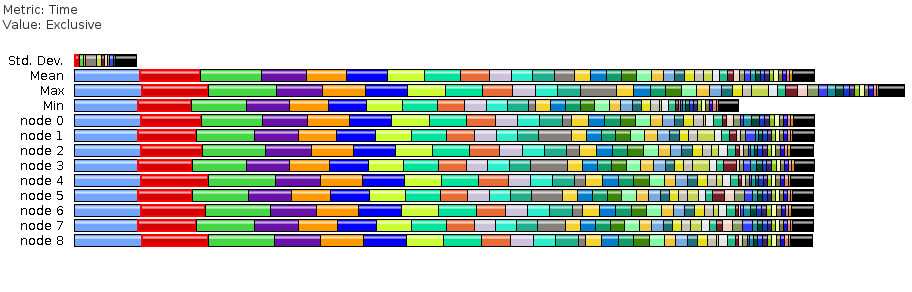
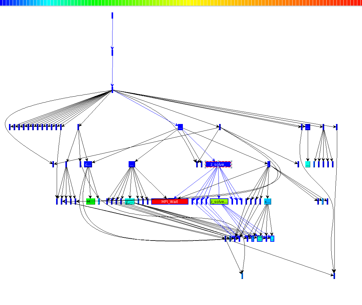
Paraprof offers visualization of the data in multiple, connected ways. For instance, one call also show the call graph of the application, which shows the runtime relationship and timings of each function.
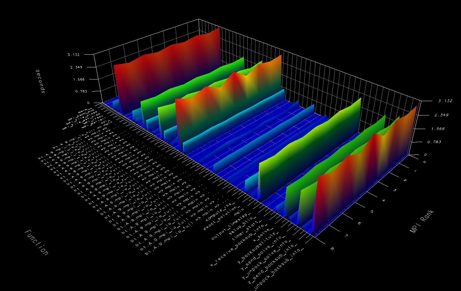
In addition, one can also generate 3D views that map MPI rank, function, and time spent.
Other views such as barcharts and histograms are available. We refer the user to the complete ParaProf documentation for further details.
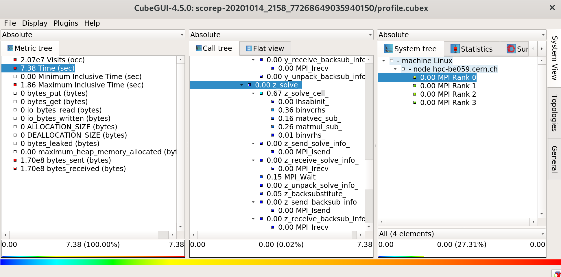
The CUBE tool is another visualization tool (the one that gives the file format its name, actually) that can be used to inspect profile data. It provides a practical way to explore the call tree, as it combines three different views (arranged into three columns) of the data: Metric tree (the kind of performance metric, e.g. Time or bytes sent), Call tree (where in the call path), and System tree (how the time is spent across processes in different machines).